Why Gaussian Latents? Deriving the Gaussian from Maximum Entropy

Introduction

Recently I have been trying to understand the motivations behind the various distributions we apply from simple games to machine learning. During this exploration, I revisited the Variational AutoEncoder (VAE), a model commonly incorporated into modern video generation models (the stuff behind the plethora of slop now contaminating my Reels). And I wondered: the standard treatment of VAEs starts from a Gaussian and inherits its parameters, but what if we ran it backwards? Suppose all we had decided was that the encoder should emit a latent mean and variance (location and scale of uncertainty) for each input. In this case, would we still get the Gaussian?

If this doesn’t make much sense, don’t worry. I will introduce the basics of the VAE and its motivations, but venture no further than the exposition necessary to understand my central question: given a mean and a variance, why choose the Gaussian distribution?

---

Compression

Unsurprisingly, the video generation techniques behind one’s realistic AI girlfriends and boyfriends are extremely complex and computationally expensive. In fact, naive generation techniques would immediately falter. One frame in a video with a 1080p Full HD resolution contains over 6 million scalar values ($1920 \cdot 1080\cdot3$), rendering generation over even a few seconds computationally infeasible, or immensely expensive.

Therefore, a common strategy in modern video generation is to compress the video into a much smaller latent representation before performing the expensive generative modeling. It’s important to consider why compression is viable here: we can postulate that it’s feasible because we’re working with frames that are consistent with the reality we observe, rather than pure pixel noise. That is, the space of reality has exploitable structure and pattern compared to random pixels.

AutoEncoders

AutoEncoders have long existed to solve this problem. They attempt to reconstruct their inputs through an information bottleneck, which becomes the latent “code” representing an input.

Then, video generation models can simply work in the much smaller latent space rather than the pixel space. (For instance, consider a model which generates autoregressive latent frames instead of full pixel frames).

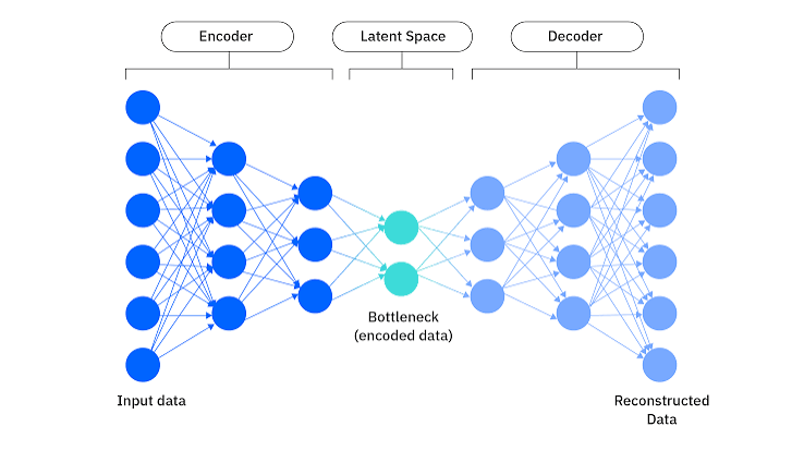
However, an issue arises with video generation: We want similar inputs to be mapped near each other in latent space, so that some amount of variation in the latent doesn’t drastically change the decoded output; however, standard AutoEncoders have no obligation to ensure this, they can simply assign each input to an isolated point in latent space, and the space between those points can be wildly meaningless.

VAEs

Thus, we enter the Variational AutoEncoder (VAE).

A VAE attacks this problem by replacing the deterministic point code with a distribution over possible latent codes, while also regularizing these distributions so that the latent space has global structure. We’ll ignore the second part and focus on the first.

Rather than declaring that an input has exactly one latent representation $z$, we can say that its representation lies somewhere within a region of latent space. A common VAE parameterization describes this region using a mean and variance—conceptually, a point in space and a scale of uncertainty:

$$\mu_\phi(x),\quad\sigma^2_\phi(x)$$

Then, to retrieve a deterministic latent code, it samples $z$ around that location.

Note on VAEs

Though VAEs are one of the common compression methods used explicitly in models such as Wan or Hunyuan Video, there are various other methods of compression that SOTA video generation models use.

So let’s try to be clear about the mathematical objects we are dealing with:

1. $p_\theta(x\mid z)$: the decoder we learn parameterized by $\theta$, where x denotes images and z denotes latents
2. $p_\theta(z\mid x)$: the true posterior representing the distribution over possible latent codes for an image
3. $p(z)$: our prior distribution over latents
4. $q_\phi(z\mid x)$: the encoder we learn parameterized by $\phi$, meant to model (2), which is intractable to compute

Note that (1) (2) and (3) are related through Bayesian inference: $p_\theta(z\mid x)=\frac{p_\theta(x\mid z)p(z)}{p_\theta(x)}$. In practice, we choose a prior and learn the decoder (1) and encoder (approximate posterior, 4), as computing the true posterior is intractable.

Let’s look at our encoder for now. Since we have decided to represent our latents with a mean and variance, it seems obvious to choose our latents to be Gaussian. Following this reasoning, our encoder takes the form of

$$q_\phi(z\mid x)= \mathcal{N}(\mu_\phi(x),\sigma^2_\phi(x)),$$

where $\mu_\phi$ and $\sigma^2_\phi$ are functions that produce a mean and a variance for an input, parameterized by $\phi$.

But is it really so obvious that we should choose the Gaussian distribution? How about we consider a few other distributions following a similar form:

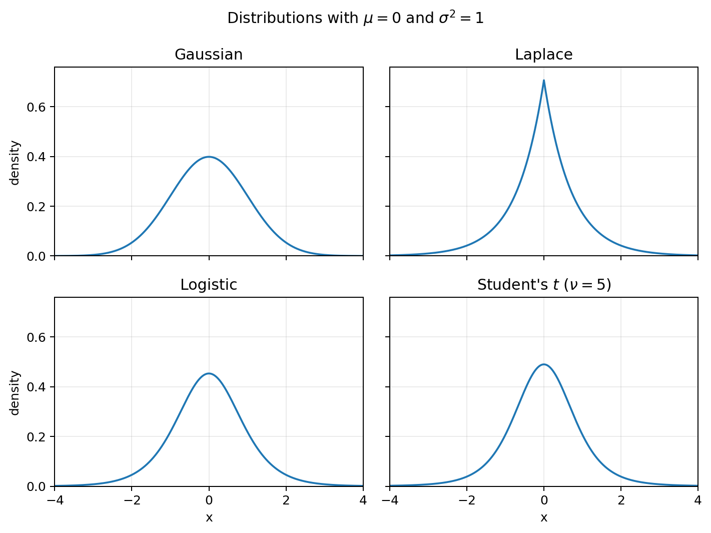
For instance, what if we used the Laplace distribution instead, with pdf:

$$f(x)=\frac{1}{\sigma\sqrt{2}}\exp\left(-\frac{\sqrt{2}|x-\mu|}{\sigma}\right)$$

Or maybe something smoother like the Logistic:

$$f(x)=\frac{\exp\left(-\frac{x-\mu}{s}\right)}{s\left[1+\exp\left(-\frac{x-\mu}{s}\right)\right]^2},\quad s=\frac{\sqrt{3}}{\pi}\sigma$$

Or maybe the Student’s t-distribution with $\nu=5$ degrees of freedom:

$$f(x)=\frac{8}{3\pi\sqrt{3}\sigma}\left(1+\frac{(x-\mu)^2}{3\sigma^2}\right)^{-3}$$

Each of these distributions can be parameterized by a mean and variance, and we can choose ones that look roughly like our standard bell-curve Gaussian.

Just for the fun of it, we can even consider some symmetric Gaussian mixture, for which one example can look like:

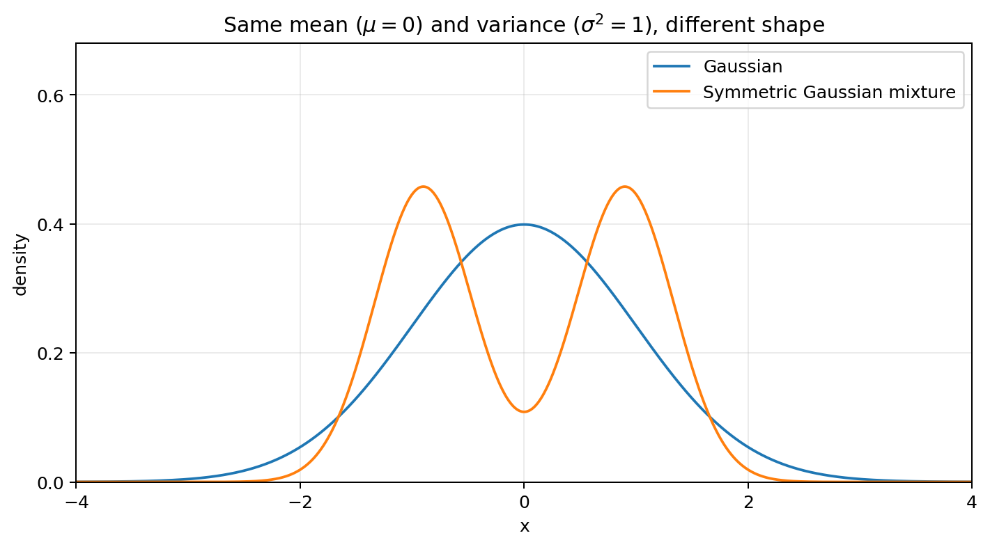
Which can be expressed by the pdf:

$$f(x)=\frac{1}{2\sigma\sqrt{2\pi(1-a^2)}}\exp\left[-\frac{(x-\mu+a\sigma)^2}{2(1-a^2)\sigma^2}\right]+\frac{1}{2\sigma\sqrt{2\pi(1-a^2)}}\exp\left[-\frac{(x-\mu-a\sigma)^2}{2(1-a^2)\sigma^2}\right]$$

The above example uses $a=0.9$, representing $X\sim \frac{1}{2}\mathcal{N}(-0.9,0.19)+\frac{1}{2}\mathcal{N}(0.9,0.19)$.

This feels pretty convoluted and seems rather complex, so maybe let’s not use it. But the point is: given a mean and variance, there are so many distributions we can choose; yet, why should we choose the Gaussian?

---

Why Gaussian?

The answer, apparently, cannot come from the mean and variance alone. Those two quantities constrain a distribution, but they do not uniquely determine its shape. Thus, we’ll need some additional principle to help us through our dilemma.

One possibility is to choose the distribution that assumes as little as possible beyond the information we were given. In other words, among all distributions with the specified mean and variance, we want the one that remains maximally uncertain everywhere else.

Let’s take a moment to break down what this means with the following steps of intuition:

1. The mean and variance are the only information we have about the distribution
2. These constraints do not uniquely determine its shape
3. We should impose as little additional, unjustified structure as possible. That is, we should aim to inject as little prior information into the distribution, and therefore be as noncommittal as possible
4. In probabilistic terms, this means remaining as uncertain as the given constraints allow
5. Entropy gives us a way to quantify that uncertainty. Thus, we arrive at the principle of maximum entropy: maximize entropy subject to the known constraints

Steps (1) and (2) are precisely what the preceding examples demonstrated. Step (3) is subtler because “additional structure” is difficult to quantify directly. We can nevertheless see that the Laplace distribution has a sharp peak, while the Gaussian mixture asserts the existence of two modes. So, we call upon Information theory to turn this intuition into something precise: entropy measures expected surprise, and maximizing entropy subject to our constraints formalizes the idea of remaining as noncommittal as possible.

Information Theory Refresher

As a quick refresher, let’s discuss some basics of Information Theory (though I think it would be good to be familiar with its principles).

Self-Information

$$I(x)=-\log p(x)$$

$I(x)$ is the self-information of an event, which we can also intuit as surprise. Intuitively, the more rare an event is, the more information we gain from it. For instance, HR asking you to meet with them is (hopefully) a low probability and (unfortunately) high information event.

Entropy

$$H(X)=\mathbb{E}[I(X)]$$

$H(X)$ is the entropy of a distribution or random variable, which we can intuit as the average surprise, or uncertainty, we have regarding the distribution.

For instance, consider discrete entropy:

$$H(X)=\sum_i{-p_i\log p_i}$$

A deterministic (one-hot) random variable has zero entropy, whereas the uniform distribution has the highest entropy among distributions with N discrete outcomes (attains entropy $\log N$). (If you would like to prove the latter argument, consider Jensen’s Inequality for a concave function, or return to this problem using the tools I introduce later).

For each outcome being as likely (and unlikely) as any other outcome, the uniform distribution intuitively has the least amount of structure, and the most amount of uncertainty.

We can also apply the same principle to continuous distributions, wherein we employ differential entropy:

$$h(X)=-\int_{-\infty}^{\infty}{f(x)\log f(x)dx}$$

Technical note: Differential Entropy Cautions

Unlike discrete entropy, differential entropy may be negative and depends on the units or coordinates used to describe X. It can still be expressed in bits or nats, but its absolute value does not have the same invariant interpretation as discrete entropy.

An interesting question now is what the maximum entropy distribution is. Unsurprisingly, over a bounded interval in $\mathbb{R}$ it is the Uniform Distribution once again, and you shall acquire the tools to prove this later. However, over all of $\mathbb{R}$, finding a maximum entropy distribution under the sole constraint of normalization ($\int_{-\infty}^{\infty} fdx=1$) has no solution (try fitting a Uniform Distribution to $(-\infty,\infty)$ and you may encounter some troubles). Therefore, additional constraints are necessary.

In our case, these constraints are precisely the mean and variance. We can therefore ask: among all probability densities on $\mathbb{R}$ with mean $\mu$ and variance $\sigma^2$, which one has the greatest differential entropy?

---

Deriving the Gaussian Distribution

Problem Setup:

$$\max_f\quad{-\int_{-\infty}^{\infty}}{f(x)\log f(x)dx}$$ $$\text{subject to}\quad\int_{-\infty}^{\infty}f(x)dx=1,\quad\int_{-\infty}^{\infty}xf(x)dx=\mu,\quad\int_{-\infty}^{\infty}x^2f(x)dx=\mu^2+\sigma^2$$

The maximization objective is just the differential entropy. Our constraints are naturally normalization, the mean $\mathbb{E}[X]=\mu$, and the variance put in the form of the second moment via the identity $\mathbb{E}[(X-\mu)^2]=\mathbb{E}[X^2]-\mu^2=\sigma^2$.

Before we try and tackle this problem analytically, let’s try employing some numerical methods to see if we really get something like a Gaussian.

Numerical Solving

Since we would like to use numerical methods, we should translate the problem to some discrete points and tackle the optimization problem there (numerical optimization over $\mathbb{R}$ would be infeasible).

For simplicity, let’s use the standardized constraints $\mu=0, \sigma^2=1$.

Discretizing the Real Line

First, we choose $N$ equally spaced grid points:

$$x_1,\ldots,x_N$$

over some sufficiently wide interval $[-L,L]$. I’ve chosen $N=61, L=6$ for experimentation.

We then associate each grid point $x_i$ with a probability mass $p_i$, where

$$p_i\geq 0,\quad\sum_{i=1}^N p_i=1$$

It is important to distinguish this $p_i$ from the probability density. The value $p_i$ represents the probability assigned to a small interval of width $\Delta x$ around $x_i$. Consequently:

$$p_i\approx f(x_i)\Delta{x}$$

Our constraints then become:

$$\sum_{i=1}^N{x_ip_i}=0,\quad\sum_{i=1}^N{x_i^2p_i}=1$$

Thus, the computer searches over every discrete probability distribution on our grid whose mean is zero and whose variance is one.

Discretizing Differential Entropy

We should also ensure that our discrete objective actually approximates differential entropy. Using

$$p_i\approx f(x_i)\Delta{x}$$

we obtain the Riemann sum approximation:

$$\begin{align*} h(X)&=-\int f(x)\log f(x)dx \\ &\approx-\sum_{i=1}^N{f(x_i)\log f(x_i)\Delta{x}}\\ &=-\sum_{i=1}^N{p_i\log \frac{p_i}{\Delta{x}}}\\ &=-\sum_{i=1}^N{p_i\log p_i}+\log\Delta x \end{align*}$$

The last line is justified by expanding the logarithm and utilizing $\sum_{i=1}^Np_i=1$.

Technical note: the reference measure

The principle of maximum entropy is nuanced when considering measures. Throughout the continuous discussion, I define densities relative to the standard Lebesgue measure. As such, the numerical approximation inherits this choice by using bins of equal Lebesgue measure $\Delta{x}$, giving $p_i\approx f(x_i)\Delta{x}$.

Therefore, our numerical problem reduces to:

$$\max_{p_1,\ldots,p_N}\quad -\sum_{i=1}^Np_i\log p_i$$ $$\text{subject to}\quad\sum_{i=1}^N p_i=1,\quad\sum_{i=1}^N x_ip_i=0,\quad\sum_{i=1}^N x_i^2p_i=1,\quad \forall_i p_i\geq 0$$

Solving with CVXPY

We can express this problem directly using CVXPY as it’s a convex optimization problem (maximizing the concave entropy objective subject to constraints is still a convex optimization problem):

x = np.linspace(-6, 6, 61)
p = cp.Variable(len(x), nonneg=True)

constraints = [
    cp.sum(p) == 1,
    x @ p == 0,
    (x**2) @ p == 1,
]

objective = cp.Maximize(cp.sum(cp.entr(p)))
problem = cp.Problem(objective, constraints)
problem.solve()

Results

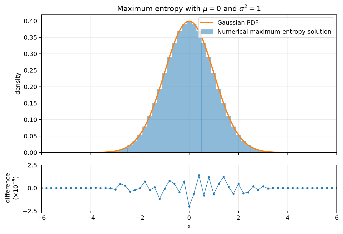
Tada! It turns out we do get something quite like a Gaussian, and the error is quite small (on the order of 1e-5).

You can probably guess now that we do actually derive the Gaussian from this maximum entropy framework, as I’ve been leading on. So let’s get to the point and derive it analytically!

Analytical Solution

I’ll reiterate the problem setup here for simplicity:

$$\max_f\quad{-\int_{-\infty}^{\infty}}{f(x)\log f(x)dx}$$ $$\text{subject to}\quad\int_{-\infty}^{\infty}f(x)dx=1,\quad\int_{-\infty}^{\infty}xf(x)dx=\mu,\quad\int_{-\infty}^{\infty}x^2f(x)dx=\mu^2+\sigma^2$$

Let’s notice that this form seems quite like something you would face in a multivariable calculus course, where you would apply Lagrange Multipliers to reduce a constrained optimization problem into an unconstrained optimization problem. The tricky part here is that unlike standard Lagrange Multiplier approaches, we are not trying to find specific variables which maximize our objective, but rather trying to find a function. Thus, we must follow by employing Calculus of Variations.

Calculus of Variations

The unifying object of Calculus of Variations is the functional. Whereas a function maps a domain to a range, a functional maps a function to a scalar value. This framing enables us to perform optimization with functions by giving a numerical label to a function; for instance, finding the function which maximizes entropy given some set of constraints.

For instance, the canonical example is the problem of finding the curve which attains the shortest path between any two points. Obviously we know it is the straight line, but we can also express it with functionals and Calculus of Variations.

Define the functional:

$$S[y]=\int_a^b\sqrt{1+\left(\frac{dy}{dx}\right)^2}dx$$

For a choice of $y(x)$ that passes through $(a, A)$ and $(b, B)$, the above functional produces a scalar value: the path length produced by the function $y$.

Now suppose $y(x)$ is the function that attains this shortest path, let $\tilde{y}(x,\epsilon)=y(x)+\epsilon\eta(x)$ be a perturbed function, where $\eta(x)$ is any smooth function such that $\eta(a)=\eta(b)=0$.

$\tilde{y}(x,\epsilon)$ can represent almost any reasonable function that passes through $(a,A)$ and $(b, B)$, and $S[\tilde{y}(x,\epsilon)]$ gives the path length of the function. We know by definition that $S[\tilde{y}(x,\epsilon)]=S[y+\epsilon\eta(x)]$ must attain its minimum when $\epsilon=0$.

This tells us a very important stationarity condition. Consider in standard calculus what the statement “a function $f(x)$ attains its minimum at $x=0$” implies. It implies $\left.\frac{d}{dx}f(x)\right|_{x=0}=0$. Similarly now, we can say that:

$$\left.\frac{d}{d\epsilon}S[\tilde{y}(x,\epsilon)]\ \right|_{\epsilon=0}=0$$

Intuitively, we can say that function we are trying to optimize is just a perturbed version of the optimal function we seek. And for the perturbed function to be stationary, it is a necessary condition that for any “infinitesimal” perturbation we add, there is no first order change.

Standard theory will then walk you through how to solve this problem, as well as the Euler-Lagrange Equation, which I suggest to look into, but for the sake of our exploration let’s return to our problem.

Lagrangian

We’ll begin by forming the Lagrangian in the hopes of turning our constrained optimization problem into an unconstrained one. Here we use the functional Lagrangian:

$$\begin{align*} \mathcal{L}[f]=&-\int_{-\infty}^{\infty}{f(x)\log f(x)dx}+\lambda_0\left(\int_{-\infty}^{\infty}f(x)dx-1\right)\\ &+\lambda_1\left(\int_{-\infty}^{\infty}xf(x)dx-\mu\right)+\lambda_2\left(\int_{-\infty}^{\infty}x^2f(x)dx-(\mu^2+\sigma^2)\right) \end{align*}$$

Collecting all the terms:

$$\begin{align*} \mathcal{L}[f]=&-\lambda_0-\lambda_1\mu-\lambda_2(\mu^2+\sigma^2)\\ &+\int_{-\infty}^{\infty}{f(x)\left(-\log f(x)+\lambda_0+\lambda_1x+\lambda_2x^2\right)dx} \end{align*}$$

Now we can express $f(x)=f^\star(x)+\epsilon\eta(x)$ in the form of a perturbed function:

$$\begin{align*} \mathcal{L}[f^\star(x)+\epsilon\eta(x)]=&-\lambda_0-\lambda_1\mu-\lambda_2(\mu^2+\sigma^2)\\ &+\int_{-\infty}^{\infty}{(f^\star(x)+\epsilon\eta(x))\left(-\log (f^\star(x)+\epsilon\eta(x))+\lambda_0+\lambda_1x+\lambda_2x^2\right)dx} \end{align*}$$

Since differential entropy is strictly concave as a functional of $f$, we know that any feasible stationary density must attain the global maximum, so we apply the stationarity condition:

$$\begin{align*} \frac{d}{d\epsilon}\mathcal{L}[f^\star(x)+\epsilon\eta(x)]&=\int_{-\infty}^{\infty}\frac{d}{d\epsilon}\left[(f^\star(x)+\epsilon\eta(x))\left(-\log (f^\star(x)+\epsilon\eta(x))+\lambda_0+\lambda_1x+\lambda_2x^2\right)\right]dx\\ &=\int_{-\infty}^{\infty}\eta(x)\left(-\log (f^\star(x)+\epsilon\eta(x))+\lambda_0+\lambda_1x+\lambda_2x^2\right)-\eta(x)dx\\ \left.\frac{d}{d\epsilon}\mathcal{L}[f^\star(x)+\epsilon\eta(x)]\right|_{\epsilon=0}&=\int_{-\infty}^{\infty}(-1-\log f^\star(x)+\lambda_0+\lambda_1x+\lambda_2x^2)\eta(x)dx \end{align*}$$

Since this integral must equal zero for stationarity, and $\eta(x)$ may be any suitable perturbation function, it is necessary that the following holds almost everywhere:

$$-1-\log f^\star(x)+\lambda_0+\lambda_1x+\lambda_2x^2=0$$

Technical note: rigor of the variational argument

My overview of Calculus of Variations is intentionally informal. In particular, I do not precisely define the admissible perturbations $\eta(x)$, and I invoke the Fundamental Lemma of the Calculus of Variations here without developing its technical conditions.

This is why I use the wording “almost everywhere”, instead of the less precise “everywhere”.

Which gives us:

$$f^\star(x)=\exp(-1+\lambda_0+\lambda_1x+\lambda_2x^2)$$

It’s easy to tell that this is already in a Gaussian form, we just need to satisfy our primal constraints to get the canonical normalized form with the mean and variance. Note that we can rewrite this in the form of:

$$f^\star(x)=C\exp(\lambda_1x+\lambda_2x^2)$$ $$f^\star(x)=C\exp(A(x+B)^2)$$

This form is equivalent where we just have to solve for $A,B,C$ using our three primal constraints, acquired by completing the square and absorbing constants. In the following derivations I will omit most of the integration steps for simplicity, which one can find the proofs and results for online. Note that $A<0$ is required for integrability.

1. Normalization:

$$\begin{align*} \int_{-\infty}^{\infty}{C\exp(A(x+B)^2)}dx&=1\\ C\left(\sqrt{\frac{\pi}{-A}}\right)&=1\\ C&=\sqrt{\frac{-A}{\pi}} \end{align*}$$

2. Mean:

$$\begin{align*} \int_{-\infty}^{\infty}{Cx\exp(A(x+B)^2)}dx&=\mu\\ C\left(-B\sqrt{\frac{\pi}{-A}}\right)&=\mu\\ B&=-\mu \end{align*}$$

3. Variance:

$$\begin{align*} \int_{-\infty}^{\infty}{Cx^2\exp(A(x+B)^2)}dx&=\mu^2+\sigma^2\\ C\left(\left(B^2-\frac{1}{2A}\right)\sqrt{\frac{\pi}{-A}}\right)&=\mu^2+\sigma^2\\ B^2-\frac{1}{2A}&=\mu^2+\sigma^2\\ \frac{1}{2A}&=-\sigma^2\\ A&=\frac{-1}{2\sigma^2} \end{align*}$$

Plugging in these values, the pdf we derive is exactly that of the Gaussian distribution:

$$\boxed{f^\star(x)=\frac{1}{\sigma\sqrt{2\pi}}\exp\left(\frac{-(x-\mu)^2}{2\sigma^2}\right)}$$

---

Looking Back

I would like to bring in a nice quote from the wikipedia page on this principle, named the “Principle of maximum entropy”, which I highly recommend to read into further.

It states, “To choose a distribution with lower entropy would be to assume information we do not possess. Thus the maximum entropy distribution is the only reasonable distribution.”

This quote provides a concise motivation for the method. For instance, if we were to choose to use a Laplace distribution knowing the Gaussian distribution is the maximum entropy distribution under the set of constraints we impose, we would be choosing to inject additional information and structure.

That said, the Laplace distribution does fall neatly into this framework. As an exercise to the reader, you may wish to prove that the Laplace distribution is the maximum entropy distribution under the constraints

$$\mathbb{E}[X]=\mu,\quad\mathbb{E}[|X-\mu|]=b,$$

where $b$ is a pre-determined scale factor.

Moreover, you now have the tools to prove that the maximum entropy distribution with support over some bounded interval in $\mathbb{R}$ is simply the Uniform distribution.

If you choose to dive into these proofs, you may notice a similar pattern that occurs. That is, if our information takes the form

$$\mathbb{E}_f[T_i(X)]=c_i$$

then repeating the same argument gives the “Exponential Family” form:

$$f^\star(x)=\exp\left(\sum_i\lambda_iT_i(x)-A(\lambda)\right)$$

Thus, the functions appearing in our constraints appear directly in the exponent of the maximum entropy distribution. This is the general exponential family pattern underlying the Gaussian, Laplace, exponential, and many other familiar distributions.

Back to the VAE

So, does the choice of representing latents with a mean and variance lead us back to the Gaussian? As you have seen, yes! In fact, what maximum entropy gives us is a more precise answer to our original question. If the encoder summarizes its uncertainty using only a mean and variance, and we do not wish to assert any additional structure, then the Gaussian is the least-committal distribution compatible with that information. It is not merely a distribution that happens to accept two parameters; it is the unique distribution that maximizes entropy under those constraints.

What maximum entropy does not do is force a VAE to use Gaussian latents in general; VAEs can be constructed with non-Gaussian priors and approximate posteriors, and the decoder distribution is a separate modeling choice.

Scope of the VAE discussion

Standard VAE explanations motivate the Gaussian, decoder, and prior more directly. So why go through this route of introducing the VAE instead of expressing the central question plainly?

Simply speaking, I stumbled upon much of the mathematics here from the initial question about VAEs, which I find rich in ideas. While you may simply ask what distribution is best given only a mean and a variance, I find the question unsatisfying, as it’s not so obvious when you would want to choose a mean and variance parameterization first, then subsequently find an appropriate distribution. I believe the core motivations of the VAE are digestible without much prerequisite knowledge, and provide a nice ML application to the central question.

The Gaussian is also particularly convenient in practice, as samples can be written in the reparameterized form

$$z=\mu_\phi(x)+\sigma_\phi(x)\odot\epsilon,\quad\epsilon\sim\mathcal{N}(0,I),$$

and its KL divergence from a standard Gaussian prior has a simple closed form.

In conclusion, this piece has motivated and covered a question leading from VAEs to probability distributions, to information theory, and finally to a derivation of one of the most familiar objects in mathematics: the Gaussian.

I find it fascinating how much valuable mathematics sits within machine learning. Through this entire piece, I have touched only on the VAE, and only as far as it was necessary to understand the maximum entropy Gaussian derivation. That said, there is still much to reap from that which has already been sown. I suppose that even in the depths of AI slop you may find the occasional gem.